Why go open?

I think the first time I ranted publicly about publishing was during Epidemics6. At the time, I was making a plea for open software practices in science, which most people seem now to agree on: transparent, free, reproducible science seems to be the way forward. Practicing my talk for this conference organised by a large publishing company, I realised these ideals were thrown away in one of the most important aspects in a researcher’s life, the publication of peer reviewed papers. Back then, I tried to outline quickly why I thought we could do better and added a few slides to my talk, which then caused a bit of laughter, and some interesting follow-up conversations. In this post I’ll try to briefly explain why I think the current dominating publishing pratice is not working, and how we can make it better.

Scientific publishing: a terrible business model

This is the easy part. While open-access journals are becoming more common, there is still a large number of journals charging for accessing their content. In short: you can access to science if you can afford it. This is the very contradiction of the idea of a science open to all. It is also poor value for money for society as a whole, due to a fairly immoral business model:

  • scientists pay to provide the very material publishers make money from
  • scientists then pay again, via their academic institutions most of the time, to gain access to content
  • the heavy lifting in the publishing industry (reviewing, editing) is made by scientists, most of the time working for free
  • as science is often publicly funded, this is effectively a stream of money going from taxpayers to private companies, without any benefit for society; it only makes science less accessible

This model is quite hard to defend whilst keeping a straight face. In fairness, it is also probably dying, as open-access journals are becoming more popular. I would argue open-access good, but open publishing (i.e. published reviews, disclosed referees) is better.

Closed review: a culture of abuse

Social psychology has studied intensively the determinants of abusive behaviour, especially in relation to hierarchical dynamics and authority (e.g. Haney, Banks, and Zimbardo 1972, Milgram (1965), Milgram (1963)). See Zimbardo (2011) for an accessible introduction to the field, and (Aronson 2003) for a deeper introduction to social psychology in general.


Figure: The Milgram experiment (Milgram 1965), a seminal study of the determinants of abusive behaviour and obedience to authority.

In (very) short: under specific circumstances, most people will engage in abusive behaviours.1 Various external factors may shape such circumstances, but amongst the most common one we often find:

  1. being in a position of power
  2. impunity
  3. having a tier holding authority held responsible for the perpetrator’s actions
  4. deriving a personal gain from the abuse
  5. having been a victim of abuse yourself

Now, if you try thinking about these in an anonymous reviewing process, you will find all the of above apply. Referees are in a position of power with respect to authors. Anonymity gives them impunity. An editor is officially in charge. Referees often review work of their perceived competitors, so they have an interest in stalling or blocking their work. And everyone who ever submitted a paper has had some horror stories about poor or unfair reviewing: a paper half read by a referee who asks for material already present, insulting or derogatory comments, stalling papers, and unsubstantiated claims, i.e. not passing the basic test of standard scientific practices.


Open review as a step forward

Most of the factors described above hinge on the fact that referees are anonymous, and usually not held accountable for their work as a referee. The solution is an easy one: make the reviewing itself an integral part of transparent scientific practices. Publish reviews alongside papers, as well as several revisions of the manuscript so that one could track how things evolved during the peer review process. Derive metrics to reward constructive and helpful reviews, and make it part of the way scientists are evaluated (is there an R-index yet?).

I won’t claim this system is without fault, but so far every argument I have heard against it have a far worse counterpart in the existing system. Open review is common practice in software development (code reviews) where it is a very useful instrument for improving work collaboratively. And an increasing number of journals such as F1000 and BMC are now using open reviews. In the age of open data, open software and open science, fully open publishing seems to be the only reasonable way forward.

References

Aronson, E. 2003. Readings About the Social Animal. Macmillan.

Haney, C, C Banks, and P Zimbardo. 1972. “Interpersonal Dynamics in a Simulated Prison.” Stanford Univ Ca Dept Of Psychology.

Milgram, S. 1963. “BEHAVIORAL STUDY OF OBEDIENCE.” J. Abnorm. Psychol. 67 (October): 371–78.

———. 1965. “Some Conditions of Obedience and Disobedience to Authority.” Hum. Relat. 18 (1). SAGE Publications Ltd: 57–76.

Zimbardo, P. 2011. The Lucifer Effect: How Good People Turn Evil. Random House.


  1. at this stage most people think ‘not me’ (I did), which usually means ‘especially you’

Ebola outbreak: what can we say with limited data?

Context

Disclaimer: this blog post only represents my views, and not that of my institution or my collaborators.

On the 8th May 2018, the Ministry of Health of the Democratic Republic of the Congo (DRC) has notified the WHO of two confirmed cases of Ebola virus disease (EVD) reported in the Bikoro health zone, Equateur province. While the WHO and the international community seems to have reacted very quickly to the situation, data in the early stages of an outbreak are always scarce. As of the writing time of the post, WHO has published a timeline of counts of cases by dates of reporting, with a total of 27 cases (including confirmed, probable or suspected cases), reported over a period of 10 days (5th - 15th May 2018).

Importantly, these data are not dates of infections, or onset (i.e. when people start showing symptoms). Therefore, at this stage it is hard to use this information for making predictions of future trajectories of the outbreak.

What do we know from past outbreaks?

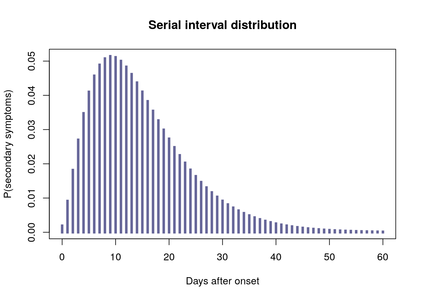
However, we do have some information on past EVD outbreaks, such as the serial interval distribution, i.e of the time between symptom onsets on a transmission chain. In other words, when a set of patients have shown symptoms and potentially infected new people, we have a statistical idea of when these new people will start showing symptoms. In the 2013-2015 EVD outbreak in West Africa, the serial interval was characterised as a discretised gamma distribution with a mean of 15.3 days, with a standard deviation of 9.3 days. We reproduce this distribution below, using the RECON packages epitrix and distcrete:

library(epitrix)
library(distcrete)

mu <- 15.3 # mean in days days
sigma <- 9.3 # standard deviation in days
cv <- sigma / mu # coefficient of variation
cv
## [1] 0.6078431
param <- gamma_mucv2shapescale(mu, cv) # convertion to Gamma parameters
param
## $shape
## [1] 2.706556
## 
## $scale
## [1] 5.652941

si <- distcrete("gamma", interval = 1,
                shape = param$shape,
                scale = param$scale, w = 0)
si
## A discrete distribution
##   name: gamma
##   parameters:
##     shape: 2.70655567117586
##     scale: 5.65294117647059

plot(0:60, si$d(0:60), type = "h", xlab = "Days after onset",
     ylab = "P(secondary symptoms)", lend = 2, lwd = 4, col = "#666699",
     main = "Serial interval distribution")

From historical data, we also have an idea of plausible values of the reproduction number \(R_0\), i.e. the average number of new cases created by an infected patient. These numbers vary widely, with central estimates ranging between 1.3 and 4.7.

Predicting future cases: the Poisson model

Taken together, the serial interval distribution and estimates of \(R_0\) can be used to estimate the force of infection (how much potential for new cases?) on a given day (example here). Typically, the number of new cases \(x_t\) on a day \(t\) is modelled as a Poisson process determined by the force of infection on that day, \(\lambda_t\), calculated as:

\[ \lambda_t = R * \sum_{s=1}^t x_s w(t - s) \]

where \(w()\) is the serial interval distribution. This can be turned into a simulation tool, which can be used to derive short term predictions of numbers of cases. This normally supposes we know dates of onsets for all cases, which we are missing here. However, we can simulate a large number of potential epidemic curves, distributing a given number of cases over a rough period of time. The function below implements this approach, relying on the RECON packages incidence and projections:

library(incidence)
library(projections)

make_simul <- function(n_initial_cases = 1, time_period = 30, n_rep = 100, ...) {
  out <- vector(length = n_rep, mode = "list")
  for (i in seq_len(n_rep)) {
    fake_data <- c(0, # index case
                   sample(seq_len(time_period),
                          n_initial_cases - 1,
                          replace = TRUE)
                   )
    fake_epicurve <- incidence::incidence(fake_data)
    out[[i]] <- project(fake_epicurve, ...)
  }

  do.call(cbind, out)
}

Caveats

Before seeing the results, please bear the following caveats in mind! These results are merely meant as a ‘what if’ scenario, used in the absence of data on this outbreak. They aim to represent plausible outcomes for an arbitrary number of cases (we don’t know exactly how many confirmed/probable cases exist in the current outbreak) having occured over an arbitrary time period (here, a month), making a bunch of assumptions, including:

  • this EVD outbreak has similar serial interval as the West African outbreak
  • \(R_0\) is within the range of past outbreaks
  • we assume an arbitrary number of 20 or 40 cases
  • we assume they occurred over a maximum period of 1 month
  • our simulations assume no impact of intervention
  • we consider an homogeneous population, wholely susceptible; in particular, we do not model the potential impact of urban settings, which would lead to increased transmissibility

Additionally:

  • we use values of \(R_0\) uniformally distributed from 1.3 to 4.7, which may give too much weight on larger values (\(R_0\) seens to be frequently <2.5, see this link)
  • we use a Poisson model, which does not account for super-spreading

Results

In the following, we look at the total number of cases which would be seen with if 20 or 40 initial cases had occured over a time period of maximum 30 days, simulating 1,000 random sets of onset dates for the initial cases, and 100 subsequent incidence curves for each (over a period of 30 days). The 100,000 resulting simulations will be summarised graphically.

Assuming 20 initial cases distributed over a month

R_values <- seq(1.3, 4.7, length = 1000)

res_20 <- make_simul(n_initial_cases = 20, time_period = 30, n_rep = 1000,
                  si = si, R = R_values, n_days = 30)
dim(res_20)
## [1]     30 100000

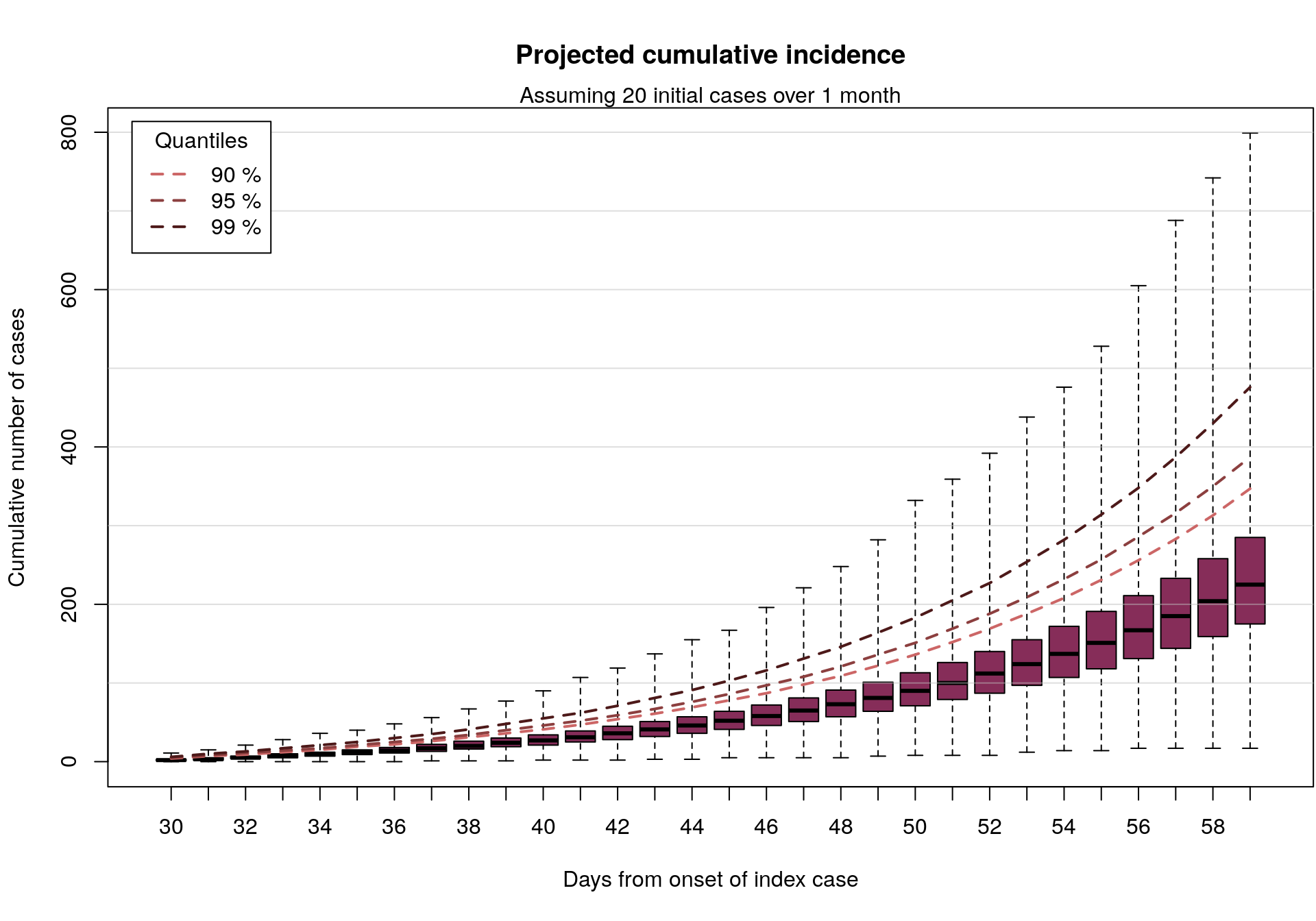
In the following graph, we represent the cumulative number of cases from 1,000 simulations, up to 30 days after the onset of the first case, assuming various values of the reproduction number (taken randomly between 1.3 and 4.7). Outliers are not displayed on these barplots but the ranges are indicated, as well as various quantiles (dashed lines).


## function to count cumulative number of cases
count_cumul_cases <- function(x) {
  out <- apply(x, 2, cumsum)
  class(out) <- c("cumul_cases", "matrix")
  out
}

## colors for quantiles
quantiles_pal <- colorRampPalette(c("#cc6666", "#4d1919"))

## function to plot outputs
plot.cumul_cases <- function(x, levels = c(.9, .95, .99), ...) {

  coords <- boxplot(t(x), col = "#862d59", xlab = "Days from onset of index case",
                    ylab = "Cumulative number of cases", outline = FALSE, range = Inf,
                    ...)

  abline(h = seq(100, 1e4, by = 100), col = "#BEBEBE80")
  quantiles <- apply(x, 1, quantile, levels)
  quantiles_col <- quantiles_pal(length(levels))
  for (i in 1:nrow(quantiles)) {
    points(1:ncol(quantiles), quantiles[i, ], type = "l", lty = 2, lwd = 2,
           col = quantiles_col[i])
  }

  legend("topleft", lty = 2, lwd = 2, col = quantiles_col,
         legend = paste(100*levels, "%"), title = "Quantiles", inset = .02)
}

## compute cumulative incidence
cumul_cases_20 <- count_cumul_cases(res_20)
dim(cumul_cases_20)
## [1]     30 100000

## plot results
par(mar = c(5.1, 4.1, 4.1, 0.1))

plot(cumul_cases_20, main = "Projected cumulative incidence")
mtext(side = 3, "Assuming 20 initial cases over 1 month")

Assuming 40 initial cases distributed over a month

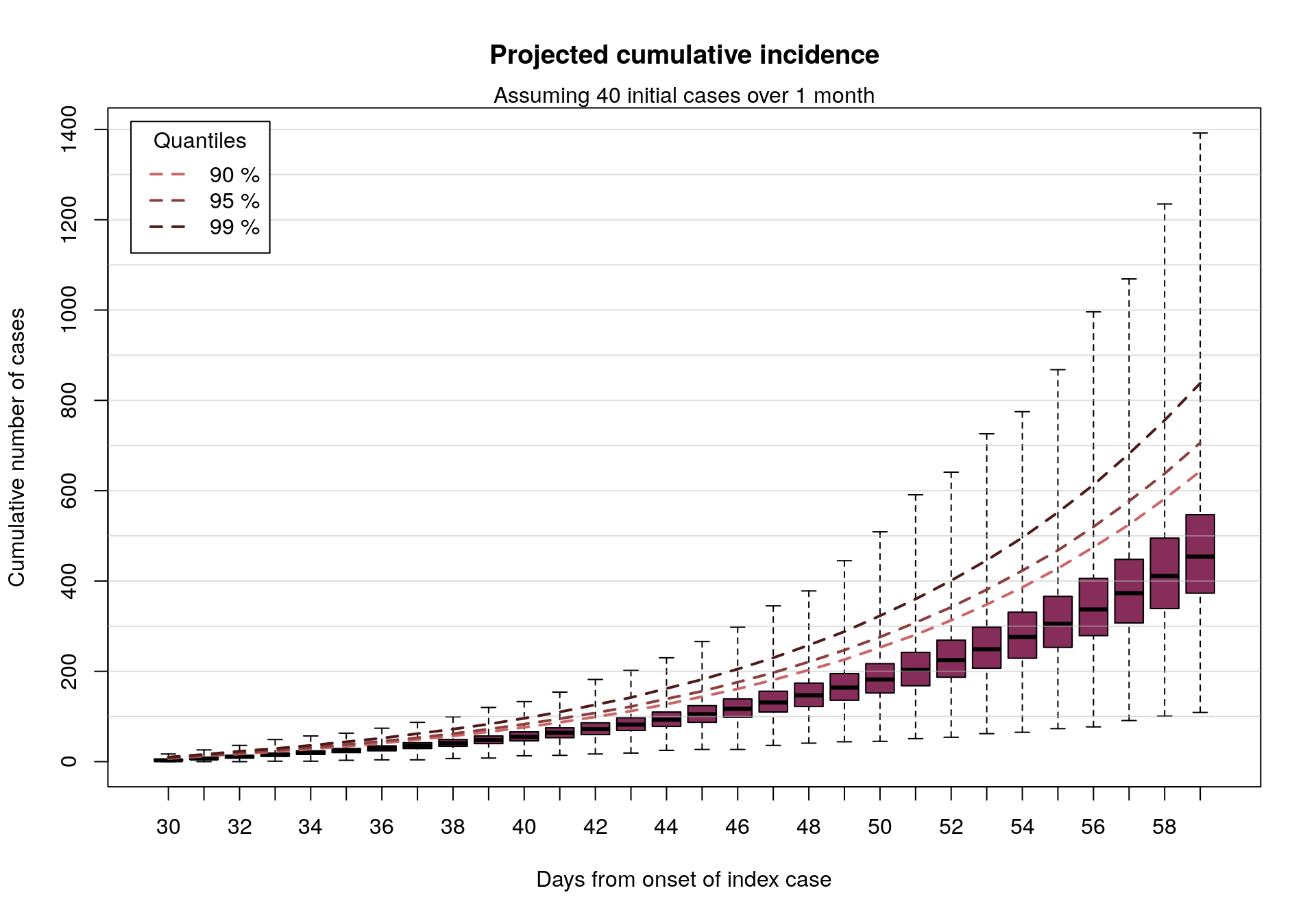
We can also look at similar results assuming twice as many cases:


res_40 <- make_simul(n_initial_cases = 40, time_period = 30, n_rep = 1000,
                     si = si, R = R_values, n_days = 30)

cumul_cases_40 <- count_cumul_cases(res_40)

plot(cumul_cases_40, main = "Projected cumulative incidence")
mtext(side = 3, "Assuming 40 initial cases over 1 month")

In short: if 20-40 EVD cases were to happen over a period of roughly 1 month, as may be the case here, and assuming an epidemiology broadly in line with previous EVD outbreaks, then in the absence of intervention we would expect to see up to a few 100s of new cases in the following month.