
Ebola outbreak: what can we say with limited data?
Context
Disclaimer: this blog post only represents my views, and not that of my institution or my collaborators.
On the 8th May 2018, the Ministry of Health of the Democratic Republic of the Congo (DRC) has notified the WHO of two confirmed cases of Ebola virus disease (EVD) reported in the Bikoro health zone, Equateur province. While the WHO and the international community seems to have reacted very quickly to the situation, data in the early stages of an outbreak are always scarce. As of the writing time of the post, WHO has published a timeline of counts of cases by dates of reporting, with a total of 27 cases (including confirmed, probable or suspected cases), reported over a period of 10 days (5th - 15th May 2018).
Importantly, these data are not dates of infections, or onset (i.e. when people start showing symptoms). Therefore, at this stage it is hard to use this information for making predictions of future trajectories of the outbreak.
What do we know from past outbreaks?
However, we do have some information on past EVD outbreaks, such as the serial interval distribution, i.e of the time between symptom onsets on a transmission chain. In other words, when a set of patients have shown symptoms and potentially infected new people, we have a statistical idea of when these new people will start showing symptoms. In the 2013-2015 EVD outbreak in West Africa, the serial interval was characterised as a discretised gamma distribution with a mean of 15.3 days, with a standard deviation of 9.3 days. We reproduce this distribution below, using the RECON packages epitrix and distcrete:
library(epitrix)
library(distcrete)

mu <- 15.3 # mean in days days
sigma <- 9.3 # standard deviation in days
cv <- sigma / mu # coefficient of variation
cv
## [1] 0.6078431
param <- gamma_mucv2shapescale(mu, cv) # convertion to Gamma parameters
param
## $shape
## [1] 2.706556
##
## $scale
## [1] 5.652941

si <- distcrete("gamma", interval = 1,
                shape = param$shape,
                scale = param$scale, w = 0)
si
## A discrete distribution
##   name: gamma
##   parameters:
##     shape: 2.70655567117586
##     scale: 5.65294117647059

plot(0:60, si$d(0:60), type = "h", xlab = "Days after onset",
     ylab = "P(secondary symptoms)", lend = 2, lwd = 4, col = "#666699",
     main = "Serial interval distribution")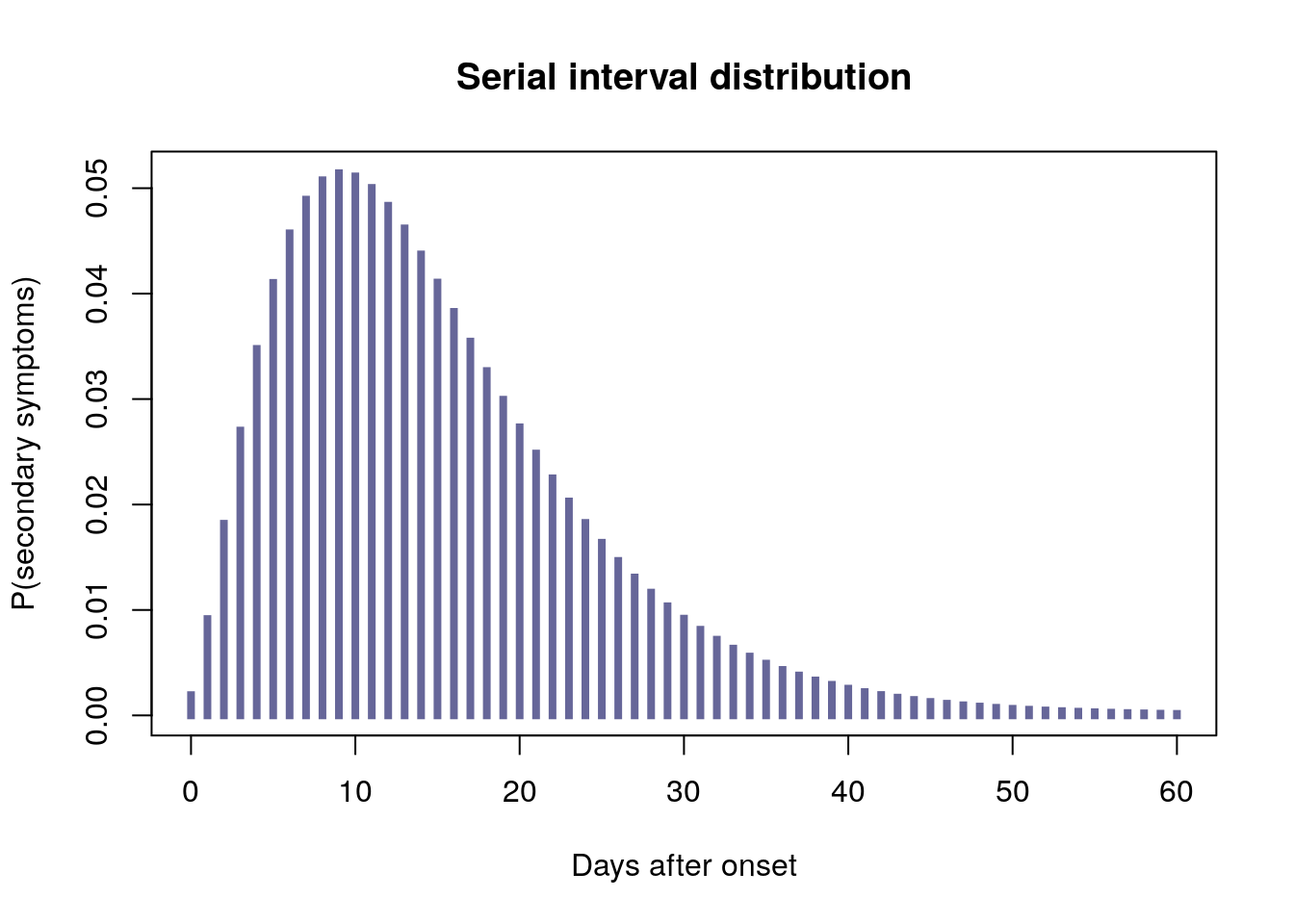
From historical data, we also have an idea of plausible values of the reproduction number \(R_0\), i.e. the average number of new cases created by an infected patient. These numbers vary widely, with central estimates ranging between 1.3 and 4.7.
Predicting future cases: the Poisson model
Taken together, the serial interval distribution and estimates of \(R_0\) can be used to estimate the force of infection (how much potential for new cases?) on a given day (example here). Typically, the number of new cases \(x_t\) on a day \(t\) is modelled as a Poisson process determined by the force of infection on that day, \(\lambda_t\), calculated as:
\[ \lambda_t = R * \sum_{s=1}^t x_s w(t - s) \]
where \(w()\) is the serial interval distribution. This can be turned into a simulation tool, which can be used to derive short term predictions of numbers of cases. This normally supposes we know dates of onsets for all cases, which we are missing here. However, we can simulate a large number of potential epidemic curves, distributing a given number of cases over a rough period of time. The function below implements this approach, relying on the RECON packages incidence and projections:
library(incidence)
library(projections)

make_simul <- function(n_initial_cases = 1, time_period = 30, n_rep = 100, ...) {
  out <- vector(length = n_rep, mode = "list")
  for (i in seq_len(n_rep)) {
    fake_data <- c(0, # index case
                   sample(seq_len(time_period),
                          n_initial_cases - 1,
                          replace = TRUE)
                   )
    fake_epicurve <- incidence::incidence(fake_data)
    out[[i]] <- project(fake_epicurve, ...)
  }

  do.call(cbind, out)
}
Caveats
Before seeing the results, please bear the following caveats in mind! These results are merely meant as a ‘what if’ scenario, used in the absence of data on this outbreak. They aim to represent plausible outcomes for an arbitrary number of cases (we don’t know exactly how many confirmed/probable cases exist in the current outbreak) having occured over an arbitrary time period (here, a month), making a bunch of assumptions, including:
- this EVD outbreak has similar serial interval as the West African outbreak
- \(R_0\) is within the range of past outbreaks
- we assume an arbitrary number of 20 or 40 cases
- we assume they occurred over a maximum period of 1 month
- our simulations assume no impact of intervention
- we consider an homogeneous population, wholely susceptible; in particular, we do not model the potential impact of urban settings, which would lead to increased transmissibility
Additionally:
- we use values of \(R_0\) uniformally distributed from 1.3 to 4.7, which may give too much weight on larger values (\(R_0\) seens to be frequently <2.5, see this link)
- we use a Poisson model, which does not account for super-spreading
Results
In the following, we look at the total number of cases which would be seen with if 20 or 40 initial cases had occured over a time period of maximum 30 days, simulating 1,000 random sets of onset dates for the initial cases, and 100 subsequent incidence curves for each (over a period of 30 days). The 100,000 resulting simulations will be summarised graphically.
Assuming 20 initial cases distributed over a month
R_values <- seq(1.3, 4.7, length = 1000)

res_20 <- make_simul(n_initial_cases = 20, time_period = 30, n_rep = 1000,
                  si = si, R = R_values, n_days = 30)
dim(res_20)
## [1]     30 100000
In the following graph, we represent the cumulative number of cases from 1,000 simulations, up to 30 days after the onset of the first case, assuming various values of the reproduction number (taken randomly between 1.3 and 4.7). Outliers are not displayed on these barplots but the ranges are indicated, as well as various quantiles (dashed lines).
## function to count cumulative number of cases
count_cumul_cases <- function(x) {
  out <- apply(x, 2, cumsum)
  class(out) <- c("cumul_cases", "matrix")
  out
}

## colors for quantiles
quantiles_pal <- colorRampPalette(c("#cc6666", "#4d1919"))

## function to plot outputs
plot.cumul_cases <- function(x, levels = c(.9, .95, .99), ...) {

  coords <- boxplot(t(x), col = "#862d59", xlab = "Days from onset of index case",
                    ylab = "Cumulative number of cases", outline = FALSE, range = Inf,
                    ...)

  abline(h = seq(100, 1e4, by = 100), col = "#BEBEBE80")
  quantiles <- apply(x, 1, quantile, levels)
  quantiles_col <- quantiles_pal(length(levels))
  for (i in 1:nrow(quantiles)) {
    points(1:ncol(quantiles), quantiles[i, ], type = "l", lty = 2, lwd = 2,
           col = quantiles_col[i])
  }

  legend("topleft", lty = 2, lwd = 2, col = quantiles_col,
         legend = paste(100*levels, "%"), title = "Quantiles", inset = .02)
}

## compute cumulative incidence
cumul_cases_20 <- count_cumul_cases(res_20)
dim(cumul_cases_20)
## [1]     30 100000

## plot results
par(mar = c(5.1, 4.1, 4.1, 0.1))

plot(cumul_cases_20, main = "Projected cumulative incidence")
mtext(side = 3, "Assuming 20 initial cases over 1 month")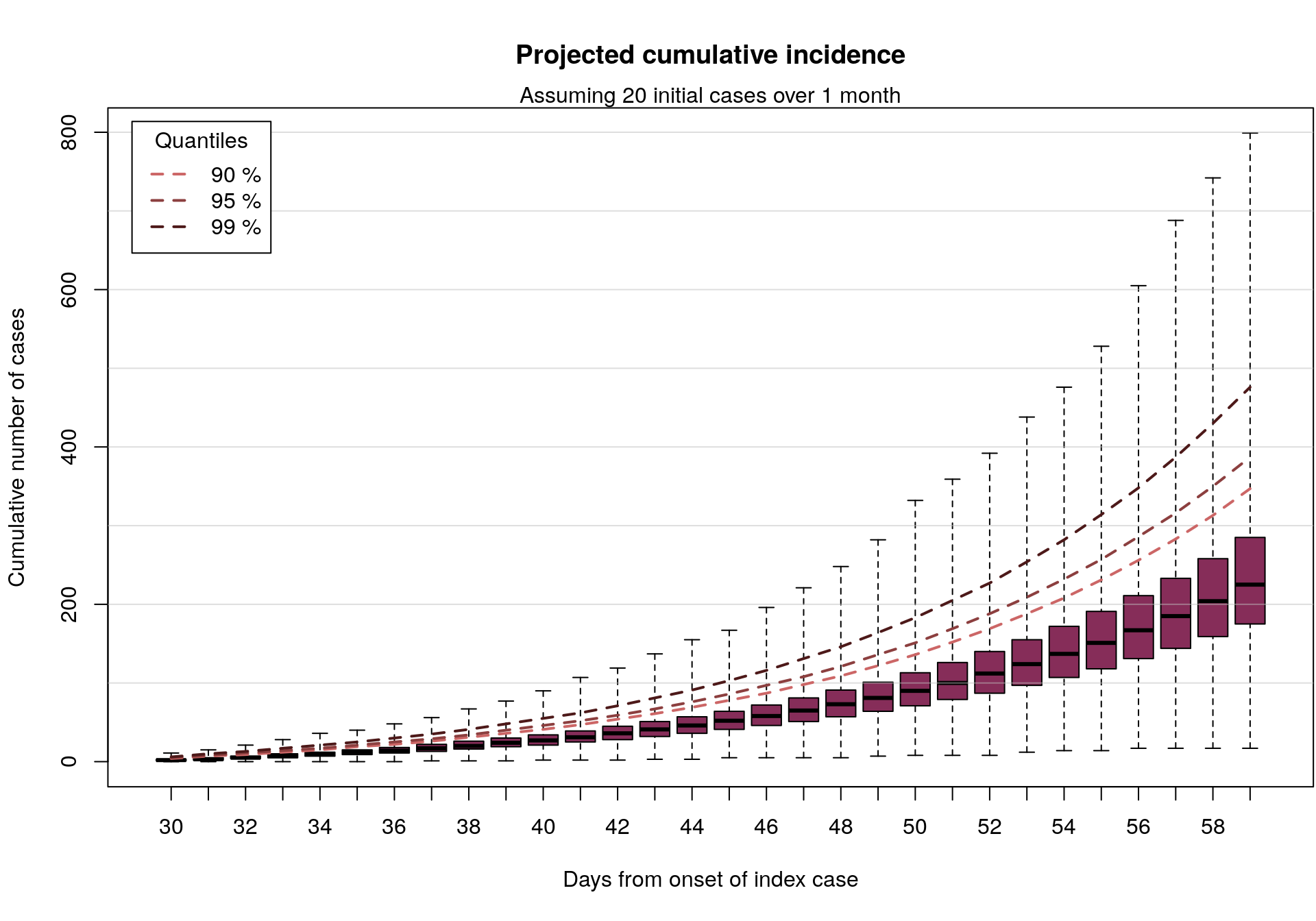
Assuming 40 initial cases distributed over a month
We can also look at similar results assuming twice as many cases:
res_40 <- make_simul(n_initial_cases = 40, time_period = 30, n_rep = 1000,
                     si = si, R = R_values, n_days = 30)

cumul_cases_40 <- count_cumul_cases(res_40)

plot(cumul_cases_40, main = "Projected cumulative incidence")
mtext(side = 3, "Assuming 40 initial cases over 1 month")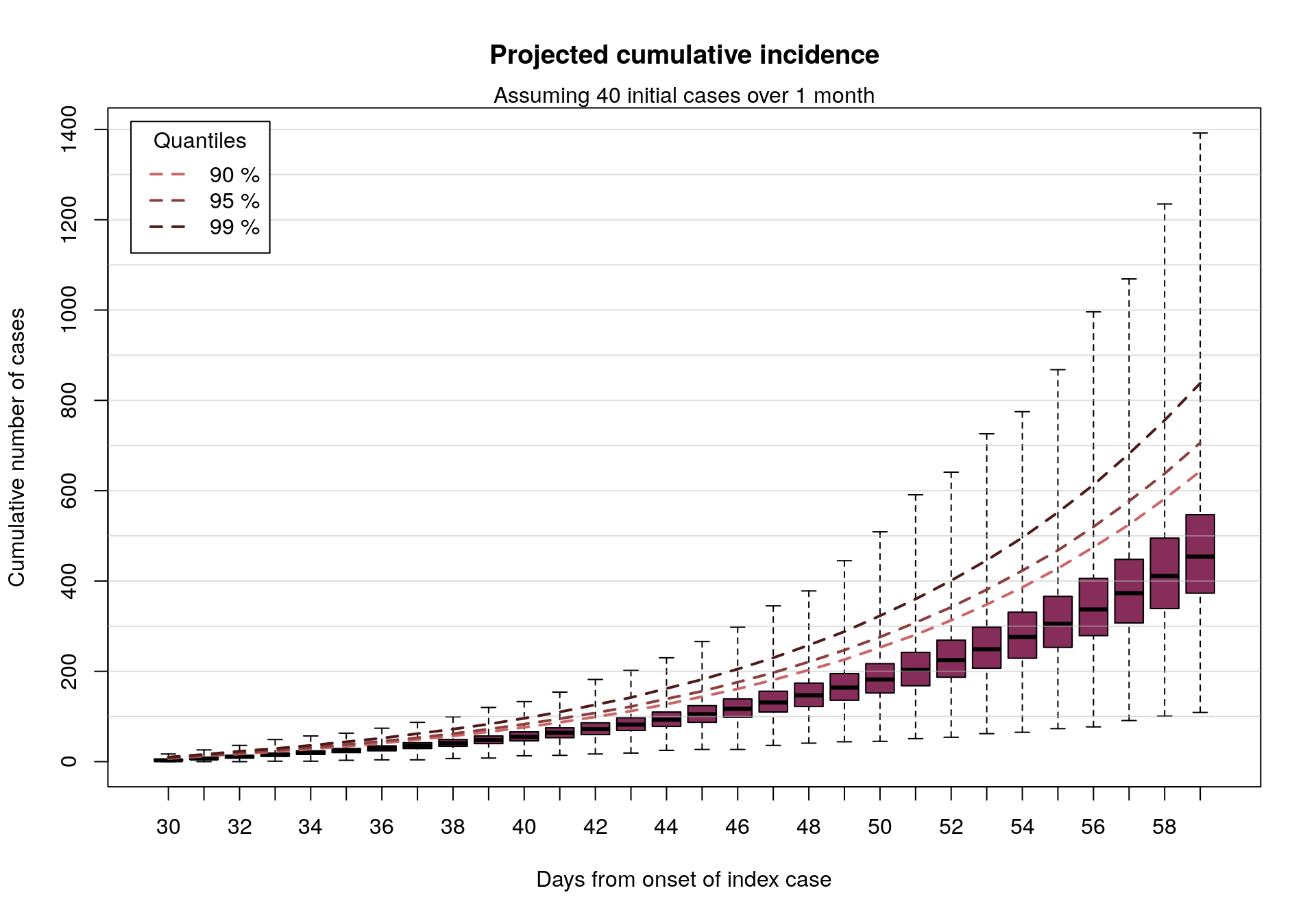
In short: if 20-40 EVD cases were to happen over a period of roughly 1 month, as may be the case here, and assuming an epidemiology broadly in line with previous EVD outbreaks, then in the absence of intervention we would expect to see up to a few 100s of new cases in the following month.